The main objective of this lab exercise is to gain a better understanding of how to perform photogrammetric tasks on satellite and aerial images. Specifically the lab is meant to teach the mathematics behind the calculation of photographic scales, calculating relief displacement and measurement of areas and perimeters of features in order for the visual analyst to gain a better understand of these topics. The overall goal is to introduce the analyst to stereoscopy and the process of performing orthorectification on satellite images.
Methods
In order to achieve the goal of this laboratory exercise and gain a better understanding of stereoscopy, orthorectification and other mathematic calculations involved in photogrammetric tasks ERDAS Imagine 2013 will be used. A more detailed explanation of each part of the lab which goes into greater detail of each process learned throughout the lab is given below.
Scales, Measurements and Relief Displacement
Calculating Scale of Nearly Vertical Aerial Photographs
Using the image below in Fig. 1, we are able to use a ruler to measure the distance from point A to point B directly from jpeg image once it is maximized on the computer screen. Once the distance is derived (2.75 inches) we can interpret the scale of the aerial photograph based on the measurement made by an engineer which found that the real distance between the points is 8822.47 ft. Based on this data we can calculate that the scale of the aerial photo in Fig. 1 is 1: 38,500" using the formula s=pd/gd (where pd is distance measured between two points in an image and gd is the real world measured distance). Next, we can calculate the scale of the photograph in Fig. 2 using the following provided information: photograph was acquired by the aircraft at an altitude of 20,000 ft above sea level with a camera focal length lens of 152 mm and the elevation of Eau Claire County is 796 ft. Using the scale formula (S= f/(H-h)) we can determine that the scale of the photograph is 1: 38, 500' (where f is the focal length lens, H is the altitude above sea level and h is the elevation of the terrain).

(Fig. 1) By measuring the distance from point A to point B in this image in inches the data can be used to determine the scale of the aerial photograph.

(Fig. 2) The scale of this aerial photograph can be determined using the photographic scale formula explained above.
Measurement of the Areas of Features on Aerial Photographs
Using the Measure tool in ERDAS Imagine 2013, we can measure the area and the perimeter of a lagoon from an aerial photograph. First, the lagoon needs to be outlined using the Polygon tool. (It is very important to make sure you outline the area precisely.) Once it has been outlined the values of the area and perimeter can be found in the measurement table below the photograph (Fig. 3).

(Fig. 3) The image above displays a lagoon in the left hand side of the image which has been outlined using the polygon tool. The values of the perimeter and area of this feature can be found in the measurement table below the image.
Calculating Relief Displacement from Object Height
As can be seen in Fig. 4 the smoke stack represented by the letter "A" has been distorted in this aerial photograph and we must determine the relief displacement of this feature. The height of the aerial camera above datum is 3,980 ft and the scale of the aerial photograph is 1:3,209. The work to determine the displacement can be found below:
Formula to use is d=
(hxr)/H and we will need to solve for h which equals the real world height
which is about 0.35 inches.
h=
(0.35)(3209)= 1123.15” r= 10.5” d= [(1123.15”)(10.5”)]/[(3980’)(12”)]= 0.246”
This tells us that the
tower is leaning away from the principle point because the value for d is a
positive number. Therefore we should make would be to move the tower towards
the principle point.

Stereoscopy is the science of depth perception using the eyes as well as other tools in order to achieve 3D viewing of a 2D image. Some of the tools that are used in stereoscopic viewing include: stereoscope, anaglyph and polaroid glasses and the development of a steromodel. In order to produce an anaglyph in ERDAS Imagine 2013, we will first need to open two images (Fig. 5) and run the Anaglyph Generation setting the DEM image (Fig. 5 right) as the DEM input image and the input image (Fig. 5 left) as the basic aerial photograph of the area. Once your output image is produced (Fig. 6), the viewer can put on polaroid glasses and observe the new image and by zooming in elevation characteristics of the anaglyph image can be seen.

(Fig. 5) The two original images that are used to produce an anaglyph image. The image on the left is an aerial photograph of the area we will be using to produce our output image and the image on the right is the DEM image which displays data referring to elevation of the same area.

(Fig. 6) Once the two original images undergo the Anaglyph Generation in ERDAS Imagine 2013, this anaglyph image is produced. (Polaroid glasses are needed to gain a better understanding of the results of this output image.)
Orthorectification
The process of orthorectification simultaneously will remove both elevational and positional errors from one or more aerial or satellite image scenes. For this process it is important to obtain the real world X, Y and Z coordinates of the pixels in the aerial photographs. In this lab, we will be using Erdas Imagine Lecia Photogrammetric Suite (LPS) which has a variety of uses. Erdas Imagine LPS can be used to extract digital and elevation models, orthorectification of images collected from a variety of sensors, digital photogrammetry for triangulation and more. For this particular portion of the laboratory exercise we will be using it to orthorectify images as well as create a planimetrically true orthoimage in the process.
Create a New Project
The first step of the project is to open LPS Project Manager in Erdas Imagine and create a new block file. To set up this file properly we need to use a polynomial-based pushbroom as the geometric model category, chose the UTM projection type, select Clarke 1866 as the spheroid name and NAD27(CONUS) as the datum name.
Activate Point Measurement Tool and Collect GCPs
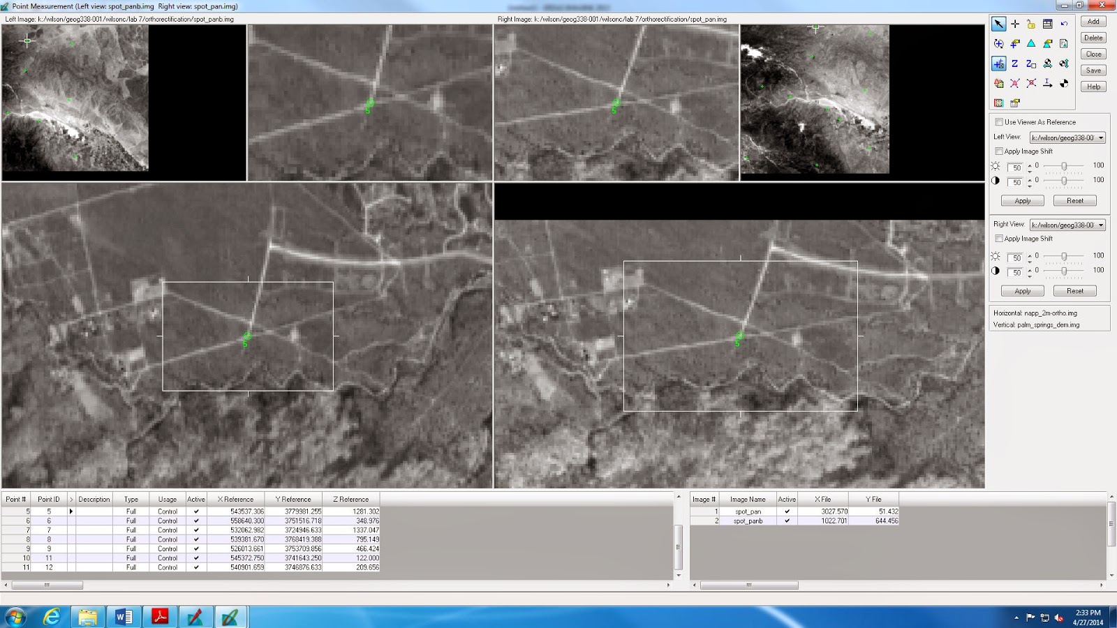
After adding the first image (spot_pan.img) to the block file the next step is to start the point measurement tool (the classic version will be used in this lab exercise). Once the point management window has opened the spot_pan.img will be displayed. We will want to change the GCP Reference Source (Horizontal reference source) first to another image in order to then use the new image as a reference in creating GCPs on our spot_pan.img. When the reference image is added, both it and the spot_pan.img will be open in the Point Management tool window. Now it is time to start collecting GCPs. To do so, we will select the point first on the reference image (Fig. 7: left) and then select the same point on the other image we are trying to orthorectify (Fig. 7: right). Once this is done the first GCP is created (Fig. 7). This process is repeated until a total of 9 GCPs have been created using the first reference image. To create the final 2 GCPs we will use a different horizontal reference source will be used. We will need to reset the horizontal reference to another image. Once that is done the final 2 GCPs can be collected (Fig. 8).

(Fig. 7) Within the Point Management tool window both the reference image (left) and the spot_pan.img (right) are shown. The green point refers to the first created GCP with the X and Y values located below the images.

(Fig. 8) The final 2 GCPs (11 and 12) are created using a different horizontal reference image but using the same process as the first 9 within the Point Management tool.
Add a Second Image to the Block and Collect its GCPs
Before adding a second image it's important to apply the "Full" formula to the Type column in the Point Management tool so that the X, Y and Z data will be used in the GCPs. Also, before adding a second image to the block we have to update the Usage column as well and make it "Control". Once that is complete a new frame can be added to the block. First close the Point Management tool and add the new frame in the LPS Project Manager. After the new image has been added to the block use the classic point management tool to collect GCPs the same way as collected the other 11. For this new image, the spot_pan.img will be used as the reference image and the newly added image to the block will be the image you will be adding new GCPs to. The point of this process is to add the points from the spot_pan.img to the new image so that they match one another (Fig. 9). This process continues until there is X and Y data for pan and panb (Fig. 9)
(Fig. 9) Now using the spot_pan.img as your reference image, a new set of GCPs can be created. As shown in the table on the bottom right side of the window, there are two sets of information, from pan and panb. Panb comes from the new image that was just added to the block.
Automatic Tie Point Collection, Triangulation and Ortho Resample
In this next part of the lab, the two images in the block will undergo processes necessary to complete the orthorectification process. The tie point collection process is used because it measures the coordinate positions of ground points within the image that appear to overlap in the two images in the block. LPS will do this process automatically and produce a summary (Fig. 10) and then any changes to the points based on inaccuracies can be made. The triangulation process also occurs automatically via LPS Project Manager as the program establishes the mathematical relationship between the images within the block file, the ground and the sensor model. It's important when conducting this process that the X, Y and Z number fields are changed to a value of 15 because of the spatial resolution of the images used in the block as this value makes sure that the GCPs are accurate to about 15 meters (Fig. 11). Once this process is run a summary is produced and a larger report can be viewed to see a more detailed description of the triangulation process (Fig. 12). The final step is to start the ortho resampling process (in LPS). Within the ortho resampling dialog, the palm_springs_dem.img will be used as the DEM which is the DTM source. In this dialog we can create two output images to reflect the two images we used in the block. After the ortho resample is run, two images will be created and can be viewed in the LPS Project Management tool window (Fig. 13).

(Fig. 10) Once a tie point collection process is run through LPS a summary will appear in the point management window which will allow the analyst to see the accuracy of the automatically produced tie points and adjust them if necessary.

(Fig. 11) This image shows the LPS Project Management window with the two images included in the block file we are using after the triangulation process has been completed.

(Fig. 12) A more detailed report of the process which LPS used to create the triangulation can be viewed from the triangulation process summary window and saved as a text file as is shown in this image.

(Fig. 13) The ortho resampling output images can be viewed in LPS Project Manager as seen in the image here.
Final Orthorectified Images
The final output images can now be viewed in ERDAS Imagine 2013. When opened in the same viewer they overlap and the area along the overlap of the two images shows how well they spatially match (Fig. 14). A more detailed view that will allow the image analyst to evaluate the overlap area in terms of spatial accuracy can be seen as we zoom into the region of overlap (Fig. 15).

(Fig. 14) The final product of the orthorectification process shows the two original images overlapping when added to the same viewer in ERDAS Imagine 2013.

(Fig. 15) A more detailed view of the area of overlap within the final, orthorectified image can be seen in the image above.
Results
The results of this laboratory exercise can be seen in the images presented throughout the methods process. Throughout this lab, the image analyst developed skills on how to calculate photographic scales, relief displacement, measure areas and perimeters of features from an aerial image and how to perform stereoscopy and orthorectification on satellite images.
Sources
The data used in this lab was provided by Dr. Cyril Wilson and collected from the following sources: NAIP in 2005 (image of Eau Claire county), aerial images of Palm Springs, California.
No comments:
Post a Comment