The goal of this lab was to better introduce analytic processes in remote sensing including:
image mosaic, band ratio, spatial and spectral image enhancement as well as binary change detection. These topics are briefly explained below.
- Image Mosaic: the combination of 2+ image scenes in order to create a single, seamless image
- Band Ratio: application of ratio transformation on an image can help to reduce environmental factors which can affect image interpretation
- Spatial Image Enhancement: used to improve the appearance of an image by amplifying subtle spectral or radiometric differences of features
- Spectral Image Enhancement: performed in order to improve an image for visual analysis by contrast enhancement
- Binary Change Detection: by subtracting the brightness values of pixels in one image and comparing them to another, this technique can be used to analyze changes in land cover over time.
By the end of this exercise, image analysts will be able to apply this practiced techniques to real world projects.
Methods:
In order to gain a firm understanding of the techniques above, ERDAS Imagine 2013 was used. The processes used to achieve the goal of the lab are presented below.
Image Mosaicking:
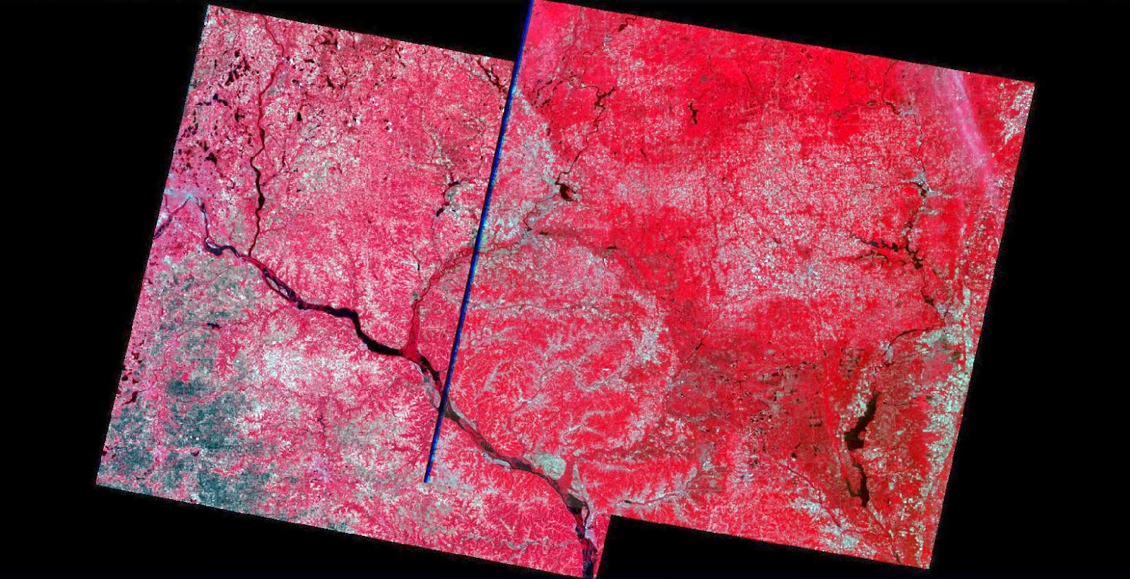
Image mosaic is used when necessary data is needed that is larger than the spatial extent of a given satellite image's area. For example, Fig. 1 shows two separate satellite images which overlap are not a mosaic but rather have just been overlapped once they were opened in ERDAS Imaging 2013. There are two ways which an image analyst can create an image mosaic in ERDAS Imagine 2013 which will be explained in greater detail below.
(Fig. 1) This is an image shows two overlapped satellite images that have yet to be formed into a mosaic.
Mosaic Express Method
Using the Mosaic Express method, we can combine the two original images in Fig. 1 in a fairly fast and simple way. The first step involves opening the Mosaic Express tool in ERDAS Imagine 2013 and selecting the images you wish to create a mosaic of. The resulting image created using this method is displayed in Fig. 2.

(Fig. 2) Mosaic of the images shown in Fig,1 using the Mosaic Express method. As can be seen in this image, the Mosaic Express method does not always produce mosaic images with a smooth color transition.
MosaicPro Method
The second technique that can produce a mosaic of the images in Fig. 1 in ERDAS Imagine 2013 is using the MosaicPro tool. This process is a bit more complex but it is a more advanced approach and produces mosaics with smooth color transitions. Once this tool is opened and the image files are imputed the viewer will display the window as shown in Fig. 3. What makes this process yield a more color accurate mosaic is the color correction step that takes place. In MosaicPro we can use the histogram matching option for color correction which will help to synchronize the radiometric properties at the region of overlap/ intersection of the two images. As a result there will be a more smooth color transition between the two image in the output image (Fig. 4).

(Fig. 3) This image shows the MosaicPro window display once the satellite image files are added.
(Fig. 4) Using the MosaicPro method to produce this mosaic image, causes there to be a smooth color transition between the two combined images compared to that of Fig. 2.
Band Ratioing:
Band ratioing uses the formula of NDVI= (NIR-Red)/ (NIR+Red) where NDVI is the normalized difference vegetation index which is one of the most widely used band ratios. The application of ratio transformations may provide unique data and information which might not have been obtained from any single band. To apply this technique, raster- unsupervised- NDVI ratio will be applied in ERDAS Imagine 2013 (Fig. 5). Within this tool it is important to make sure the function is NDVI and the the Landsat TM sensor are selected. Once the new band ratio is applied to the original image the produced image will be produced which will provide a different interpretation information than the original as shown in the comparison in Fig. 6.


(Fig. 6) This image shows the original image on the left and the output image after a NDVI band ratio was applied on the right. The changes made to the image allow for the image interpreter to see certain features once the environmental factors were reduced from the original image to produce the image on the right.
(Fig. 5) The original image is displayed with the unsupervised-NDVI tool open in ERDAS Imagine 2013. The important features of this tool for this process is the function NDVI and the Landsat TM sensor being used.
Spatial Enhancement
This section introduces two techniques used in spatial enhancement of images. The overall goal of this process is to make adjustments which amplify the spectral or radiometric differences in a feature in order to make it easier for the image interpreter to analyze. There are three main ways to apply/ perform spatial enhancements, by using spatial filtering and edge enhancement.
Spatial Filtering
Spatial filtering is used to either accentuate or suppress spatial frequencies (changes in the brightness values per unit of distance in a particular image) in remotely sensed images. Convolution filtering is based on the usage of a convolution mask to adjust the spatial frequencies of an image and are divided into two types: high pass and low pass filters. Low pass filters decrease the high spectral frequencies in an image. High pass filters remove the low frequency portions of an image and enhance the high-frequency, local variation within an image. To apply these filters to an image, the spatial convolution tool must be used as can be seen in Fig. 7. Once a filter is applied, the results can be seen in the comparison of the original image and the output image. (The results of the low-pass filter can be seen in Fig. 8 and the results of the high-pass filter can be seen in Fig. 9).

(Fig. 7) This image demonstrates the convolution tool in ERDAS Imagine 2013 which is used to apply both low and high pass filters to an image. In this particular image, a low-pass filter is being applied (which can be seen under kernel selection).

(Fig. 8) After a low-pass convolution filter was applied to the original image (left) the output produced (right) is much less clear, as this type of filter is meant to tone down the high spectral frequency of an image.

(Fig. 9) A high-pass convolution filter was applied to the original image (left) and as a result the output image (right) is much sharper once the low frequency components were removed and the high frequency variation was enhanced.
Edge Enhancement
The use of edge enhancement does exactly what the name suggests, it enhances, or delineates edges and makes the shapes and details within an image more distinct and therefore visible. This technique can be performed using two different methods, directional or laplacian convolution masks. In this lab we worked with laplacian convolution masks which locally increase the contrast at discontinuances, resulting in a sharpened image.

(Fig. 10) Using the same convolution tool in ERDAS Imagine 2013 to adjust the original image (left) but selecting the laplacian edge detection kernel, handle image by fill and unchecking the image to normalize kernel the output image (right) will be produced. As can be seen in this comparison, the output image on the right has a greater amount of contrast between the pixels than the original image.
Spectral Enhancement:
Spectral enhancement is performed to improve an image for visual interpretation via contrast enhancement. There are two main techniques to achieve this: linear and nonlinear methods. Within this lab we focused on the two linear methods of minimum-maximum and piece-wise linear contrast stretch and one non linear method which was histogram equalization. These techniques are described in greater detail below.


Spectral enhancement is performed to improve an image for visual interpretation via contrast enhancement. There are two main techniques to achieve this: linear and nonlinear methods. Within this lab we focused on the two linear methods of minimum-maximum and piece-wise linear contrast stretch and one non linear method which was histogram equalization. These techniques are described in greater detail below.
Minimum- Maximum Contrast Stretch
The minimum-maximum contrast stretch is usually best applied to images that have a Gaussian or near-Gaussian histogram which are rare in real images. This technique remaps the minimum brightness value to zero and the maximum brightness value to 255. In ERDAS Imagine 2013, we first navigate to the panchromatic- general contrast adjustment option where we use the Gaussain method (shown in Fig. 11).
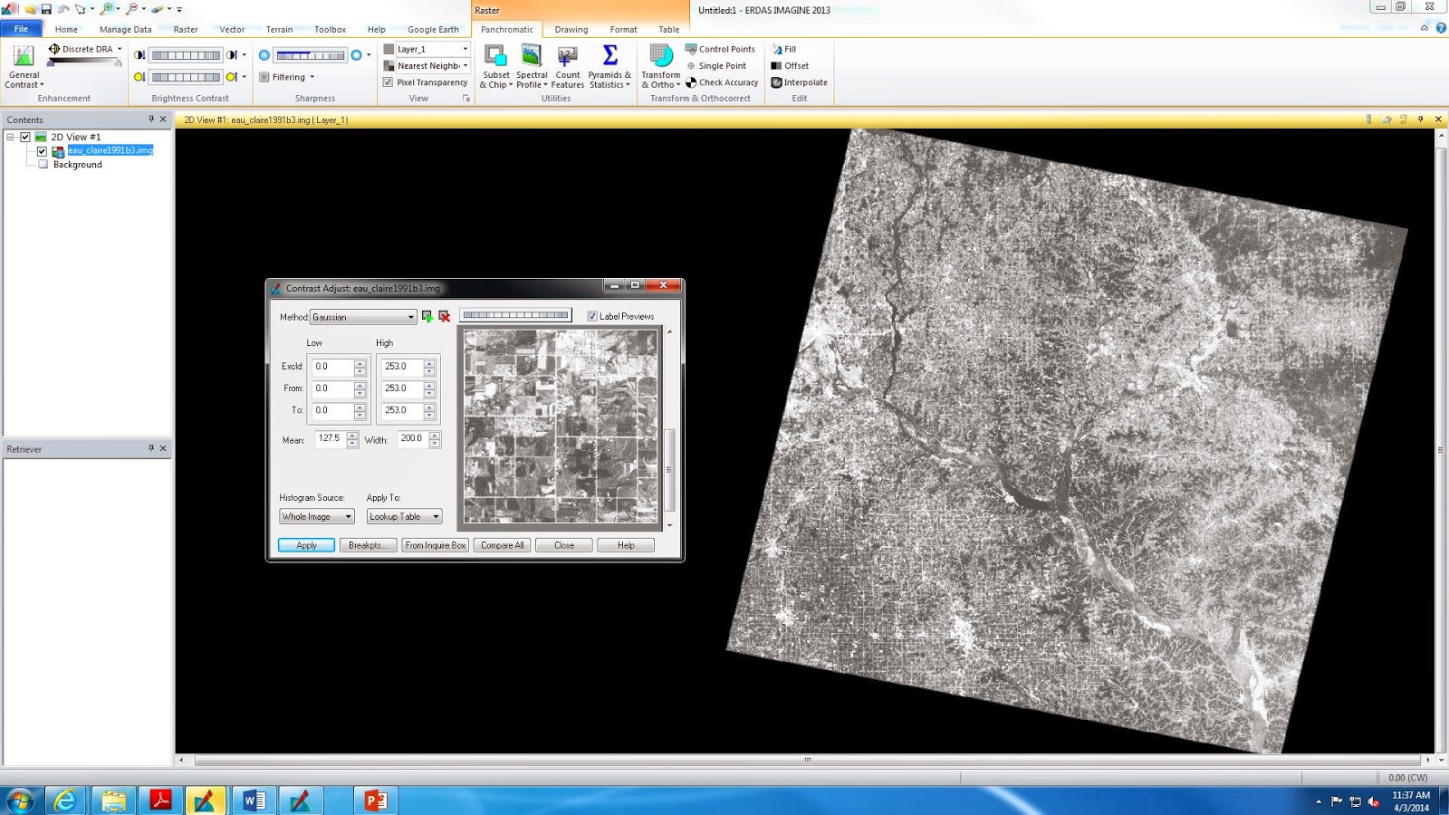
(Fig. 11) The Gaussian method is being used to perform a linear, spectral enhancement to the image on the right using the general contrast adjustment tool.
The minimum-maximum contrast stretch is usually best applied to images that have a Gaussian or near-Gaussian histogram which are rare in real images. This technique remaps the minimum brightness value to zero and the maximum brightness value to 255. In ERDAS Imagine 2013, we first navigate to the panchromatic- general contrast adjustment option where we use the Gaussain method (shown in Fig. 11).
(Fig. 11) The Gaussian method is being used to perform a linear, spectral enhancement to the image on the right using the general contrast adjustment tool.
Piece-Wise Linear Contrast Stretch
The piece-wise contrast stretch is utilized when the image's histogram is not Gaussian or multimodal. An analyst is to identify a number of linear enhancement steps to expand the ranges of the histogram. Figure 12 demonstrates the process used in ERDAS Imagine 2013 to apply this type of adjustment.

(Fig. 12) This displays the contrast tool used to apply the piece-wise linear contrast stretch.
Histogram Equalization
This technique is the only nonlinear enhancement we performed in this lab and focuses on improving the contrast to enhance visual interpretation. Once an image has the histogram equalization process applied to it the output image has a greater contrast and therefore the image analyst is able to better identify features in an image. This process can be used to study the changes in an area over time (such as in the images displayed in Fig. 13) based on the changes in pixels between images that show the same area. There are two ways to achieve this goal in ERDAS Imagine 2013. The first is by using the two input operations tool which combines images (Fig. 13) into one (Fig. 15) output image. The next method is mapping the change in pixels using the spatial modeler. This method is more complex as it uses the model maker to overlap the two original images. It shows a more clear display of how the two raster images are combined to produce a single one (Fig. 16). The final image will show the differences in the pixels between the two images from 1991 to 2011 (Fig. 17).
(Fig. 13) Both of these images display the same region but were taken at two different times. The left image was taken in 1991 and the one on the right was taken in 2011.
(Fig. 14) The two original images which were combined using the two input operation tool in ERDAS Imagine 2013 is shown here. The images are zoomed in versions of the larger images shown in Fig. 13.
(Fig. 15) This shows the output image produced from the two original images (Fig. 13) after the are combined using the two image function tool in ERDAS Imagine 2013.
(Fig. 16) The model maker tool is displayed here as a method for studying the changes in an area based on the differences in the pixels over time.
(Fig. 17) This is the resulting image produced from the model maker tool in ERDAS Imagine 2013, which directly shows the pixels which are different between the original images of the same area taken 10 years apart (Fig. 13).
Results from this lab exercise are displayed above. Through these techniques we are better able to understand the various forms of image function including spatial and spectral analysis.
Sources:
Data utilized in this lab exercise was provided by Dr. Cyril Wilson. Satellite images were captured by Landsat TM sensors.
No comments:
Post a Comment