Remote Sensing Lab 8

Goals and Background

The goal of this laboratory exercise is for the image analyst to gain a better understand and experience the collection, measurement and interpretation of spectral reflectance signatures of various surface features. These features include Earth surface and near surface materials that were photographed by satellites. Within this lab we will discuss how to collect these spectral signatures from remotely sensed images and graph them in order to analyze them and verify whether they pass the "spectral separability test". 

Methods

In this lab, we will use ERDAS Imagine 2013 to measure and plot the spectral reflectance values of 12 materials and surfaces from a remotely sensed image of Eau Claire County, WI. The following features that we will be measuring can be seen listed below:

1. Standing Water
2. Moving water
3. Vegetation
4. Riparian vegetation.
5. Crops
6. Urban Grass
7. Dry soil (uncultivated)
8. Moist soil (uncultivated)
9. Rock
10. Asphalt highway
11. Airport runway
12. Concrete surface (Parking lot)

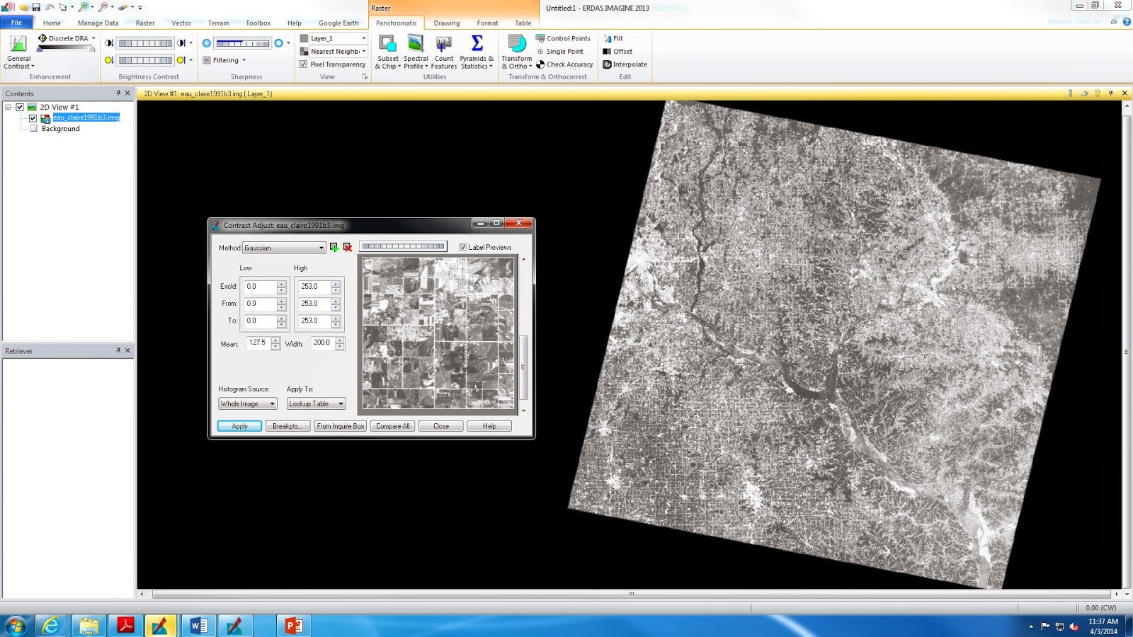
First we will open the image in ERDAS Imagine 2013 and use the drawing tool and outline the area of the feature using the polygon tool (an example can be seen in Fig. 1). Then we must activate the raster processing tools selecting the supervised and signature editor. After a feature is selected by the polygon drawing tool we will then select the option to add the "Create New Signatures from AOI" to add the selected area. Once this is done we can see a more detailed view of the Mean Plot in order to help us identify the signatures. Next all the plots can be combined into one and comparisons can be made based on the values displayed (Figs. 2 and 3).

(Fig. 1) The selected area in the standing body of water can be seen by the polygon in the body of water to the right of the two windows. The window on the left represents the Signature Editor Tool where new signatures can be added. Once the signatures are added they can be viewed in the Signature Mean Plot shown by the window to the right.

(Fig. 2) This image shows the Signature Editor Tool once all the features listed in the above methods section have been added.

(Fig. 3) This graph displays a combined Signature Mean Plot with all the features added to it so the data can be compared and analyzed.

Results

By the end of this lab then those who complete it can collect and as well as analyze spectral signatures for the various types of features in a multispectral remotely sensed image.

Sources

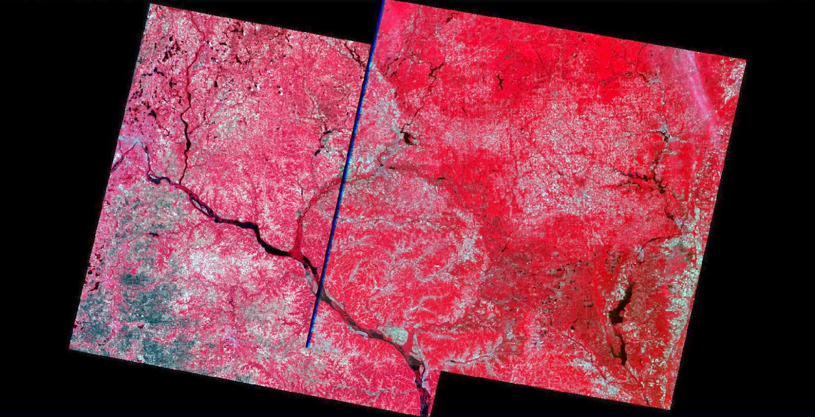
All data used in this lab was provided by Dr. Cyril Wilson. The image of Eau Claire county were collected using a Landsat ETM+ and also a selection of the Twin Cities and was taken in 2000.

Remote Sensing Lab 7

Goals and Background

The main objective of this lab exercise is to gain a better understanding of how to perform photogrammetric tasks on satellite and aerial images. Specifically the lab is meant to teach the mathematics behind the calculation of photographic scales, calculating relief displacement and measurement of areas and perimeters of features in order for the visual analyst to gain a better understand of these topics. The overall goal is to introduce the analyst to stereoscopy and the process of performing orthorectification on satellite images.

Methods

In order to achieve the goal of this laboratory exercise and gain a better understanding of stereoscopy, orthorectification and other mathematic calculations involved in photogrammetric tasks ERDAS Imagine 2013 will be used. A more detailed explanation of each part of the lab which goes into greater detail of each process learned throughout the lab is given below.

Scales, Measurements and Relief Displacement

Calculating Scale of Nearly Vertical Aerial Photographs

Using the image below in Fig. 1, we are able to use a ruler to measure the distance from point A to point B directly from jpeg image once it is maximized on the computer screen. Once the distance is derived (2.75 inches) we can interpret the scale of the aerial photograph based on the measurement made by an engineer which found that the real distance between the points is 8822.47 ft. Based on this data we can calculate that the scale of the aerial photo in Fig. 1 is 1: 38,500" using the formula s=pd/gd (where pd is distance measured between two points in an image and gd is the real world measured distance). Next, we can calculate the scale of the photograph in Fig. 2 using the following provided information: photograph was acquired by the aircraft at an altitude of 20,000 ft above sea level with a camera focal length lens of 152 mm and the elevation of Eau Claire County is 796 ft. Using the scale formula (S= f/(H-h)) we can determine that the scale of the photograph is 1: 38, 500' (where f is the focal length lens, H is the altitude above sea level and h is the elevation of the terrain).

 

 

(Fig. 1) By measuring the distance from point A to point B in this image in inches the data can be used to determine the scale of the aerial photograph.

 

 

(Fig. 2) The scale of this aerial photograph can be determined using the photographic scale formula explained above.

 

Measurement of the Areas of Features on Aerial Photographs

Using the Measure tool in ERDAS Imagine 2013, we can measure the area and the perimeter of a lagoon from an aerial photograph. First, the lagoon needs to be outlined using the Polygon tool. (It is very important to make sure you outline the area precisely.) Once it has been outlined the values of the area and perimeter can be found in the measurement table below the photograph (Fig. 3).

 

 

(Fig. 3) The image above displays a lagoon in the left hand side of the image which has been outlined using the polygon tool. The values of the perimeter and area of this feature can be found in the measurement table below the image.

 

Calculating Relief Displacement from Object Height

As can be seen in Fig. 4 the smoke stack represented by the letter "A" has been distorted in this aerial photograph and we must determine the relief displacement of this feature. The height of the aerial camera above datum is 3,980 ft and the scale of the aerial photograph is 1:3,209. The work to determine the displacement can be found below:

 

Formula to use is d= (hxr)/H and we will need to solve for h which equals the real world height which is about 0.35 inches.

h= (0.35)(3209)= 1123.15”                                                    r= 10.5”                                                   d= [(1123.15”)(10.5”)]/[(3980’)(12”)]= 0.246”     

This tells us that the tower is leaning away from the principle point because the value for d is a positive number. Therefore we should make would be to move the tower towards the principle point.

 

 

(Fig. 4) The smoke stack is indicated by the letter "A" in the upper right hand corner of the image while the principle point is in the upper left hand corner.

 

Stereoscopy

Stereoscopy is the science of depth perception using the eyes as well as other tools in order to achieve 3D viewing of a 2D image. Some of the tools that are used in stereoscopic viewing include: stereoscope, anaglyph and polaroid glasses and the development of a steromodel. In order to produce an anaglyph in ERDAS Imagine 2013, we will first need to open two images (Fig. 5) and run the Anaglyph Generation setting the DEM image (Fig. 5 right) as the DEM input image and the input image (Fig. 5 left) as the basic aerial photograph of the area. Once your output image is produced (Fig. 6), the viewer can put on polaroid glasses and observe the new image and by zooming in elevation characteristics of the anaglyph image can be seen.

 

(Fig. 5) The two original images that are used to produce an anaglyph image. The image on the left is an aerial photograph of the area we will be using to produce our output image and the image on the right is the DEM image which displays data referring to elevation of the same area.

 

 

(Fig. 6) Once the two original images undergo the Anaglyph Generation in ERDAS Imagine 2013, this anaglyph image is produced. (Polaroid glasses are needed to gain a better understanding of the results of this output image.)

Orthorectification
The process of orthorectification simultaneously will remove both elevational and positional errors from one or more aerial or satellite image scenes. For this process it is important to obtain the real world X, Y and Z coordinates of the pixels in the aerial photographs. In this lab, we will be using Erdas Imagine Lecia Photogrammetric Suite (LPS) which has a variety of uses. Erdas Imagine LPS can be used to extract digital and elevation models, orthorectification of images collected from a variety of sensors, digital photogrammetry for triangulation and more. For this particular portion of the laboratory exercise we will be using it to orthorectify images as well as create a planimetrically true orthoimage in the process.

Create a New Project

The first step of the project is to open LPS Project Manager in Erdas Imagine and create a new block file. To set up this file properly we need to use a polynomial-based pushbroom as the geometric model category, chose the UTM projection type, select Clarke 1866 as the spheroid name and NAD27(CONUS) as the datum name.  

 

Activate Point Measurement Tool and Collect GCPs

After adding the first image (spot_pan.img) to the block file the next step is to start the point measurement tool (the classic version will be used in this lab exercise). Once the point management window has opened the spot_pan.img will be displayed. We will want to change the GCP Reference Source (Horizontal reference source) first to another image in order to then use the new image as a reference in creating GCPs on our spot_pan.img. When the reference image is added, both it and the spot_pan.img will be open in the Point Management tool window. Now it is time to start collecting GCPs. To do so, we will select the point first on the reference image (Fig. 7: left) and then select the same point on the other image we are trying to orthorectify (Fig. 7: right). Once this is done the first GCP is created (Fig. 7). This process is repeated until a total of 9 GCPs have been created using the first reference image. To create the final 2 GCPs we will use a different horizontal reference source will be used. We will need to reset the horizontal reference to another image. Once that is done the final 2 GCPs can be collected (Fig. 8).

 

 

(Fig. 7) Within the Point Management tool window both the reference image (left) and the spot_pan.img (right) are shown. The green point refers to the first created GCP with the X and Y values located below the images.

 

 

(Fig. 8) The final 2 GCPs (11 and 12) are created using a different horizontal reference image but using the same process as the first 9 within the Point Management tool.

 

Add a Second Image to the Block and Collect its GCPs

Before adding a second image it's important to apply the "Full" formula to the Type column in the Point Management tool so that the X, Y and Z data will be used in the GCPs. Also, before adding a second image to the block we have to update the Usage column as well and make it "Control". Once that is complete a new frame can be added to the block. First close the Point Management tool and add the new frame in the LPS Project Manager. After the new image has been added to the block use the classic point management tool to collect GCPs the same way as collected the other 11. For this new image, the spot_pan.img will be used as the reference image and the newly added image to the block will be the image you will be adding new GCPs to. The point of this process is to add the points from the spot_pan.img to the new image so that they match one another (Fig. 9). This process continues until there is X and Y data for pan and panb (Fig. 9)

 

 

(Fig. 9) Now using the spot_pan.img as your reference image, a new set of GCPs can be created. As shown in the table on the bottom right side of the window, there are two sets of information, from pan and panb. Panb comes from the new image that was just added to the block.

 

Automatic Tie Point Collection, Triangulation and Ortho Resample

In this next part of the lab, the two images in the block will undergo processes necessary to complete the orthorectification process. The tie point collection process is used because it measures the coordinate positions of ground points within the image that appear to overlap in the two images in the block. LPS will do this process automatically and produce a summary (Fig. 10) and then any changes to the points based on inaccuracies can be made. The triangulation process also occurs automatically via LPS Project Manager as the program establishes the mathematical relationship between the images within the block file, the ground and the sensor model. It's important when conducting this process that the X, Y and Z number fields are changed to a value of 15 because of the spatial resolution of the images used in the block as this value makes sure that the GCPs are accurate to about 15 meters (Fig. 11). Once this process is run a summary is produced and a larger report can be viewed to see a more detailed description of the triangulation process (Fig. 12). The final step is to start the ortho resampling process (in LPS). Within the ortho resampling dialog, the palm_springs_dem.img will be used as the DEM which is the DTM source. In this dialog we can create two output images to reflect the two images we used in the block. After the ortho resample is run, two images will be created and can be viewed in the LPS Project Management tool window (Fig. 13).

 

 

(Fig. 10) Once a tie point collection process is run through LPS a summary will appear in the point management window which will allow the analyst to see the accuracy of the automatically produced tie points and adjust them if necessary.

 

 

(Fig. 11) This image shows the LPS Project Management window with the two images included in the block file we are using after the triangulation process has been completed.

 

(Fig. 12) A more detailed report of the process which LPS used to create the triangulation can be viewed from the triangulation process summary window and saved as a text file as is shown in this image.

 

 

(Fig. 13) The ortho resampling output images can be viewed in LPS Project Manager as seen in the image here.

 

Final Orthorectified Images

 

The final output images can now be viewed in ERDAS Imagine 2013. When opened in the same viewer they overlap and the area along the overlap of the two images shows how well they spatially match (Fig. 14). A more detailed view that will allow the image analyst to evaluate the overlap area in terms of spatial accuracy can be seen as we zoom into the region of overlap (Fig. 15).

 

 

(Fig. 14) The final product of the orthorectification process shows the two original images overlapping when added to the same viewer in ERDAS Imagine 2013.

 

(Fig. 15) A more detailed view of the area of overlap within the final, orthorectified image can be seen in the image above.



Results

 

The results of this laboratory exercise can be seen in the images presented throughout the methods process. Throughout this lab, the image analyst developed skills on how to calculate photographic scales, relief displacement, measure areas and perimeters of features from an aerial image and how to perform stereoscopy and orthorectification on satellite images.

 

Sources

 

The data used in this lab was provided by Dr. Cyril Wilson and collected from the following sources: NAIP in 2005 (image of Eau Claire county), aerial images of Palm Springs, California.

 

 

 



Remote Sensing Lab 6

Goal and Background

The goal of this lab is to introduce the preprocessing method of geometric correction. Throughout the laboratory exercise, the two types of geometric correction will be discussed and each method will be practiced.

1.Image-to-Map Rectification:

This type of interpolation transforms the image data pixel coordinates using the map coordinate components.

2. Image-to-Image Rectification:

This method is the same process of correction however; the reference image is one which has already been corrected.

Methods
In order to gain a firm understanding of the techniques above, ERDAS Imagine 2013 was used. The processes used to achieve the goal of the lab are presented below.

Image-to-Map Rectification:

Rectification is the process where a data file coordinate is converted to another grid and coordinate system, known as a reference system. Using the map coordinate counterparts the image data pixel coordinates are transformed resulting in a planimetric image. The first step in ERDAS Imagine 2013 to begin this transformation is to select the Control Points option in the Multispectral tool list. Using this tool the two images (Fig. 1) will be used to perform the image-map-rectification method of geometric correction.

(Fig. 1) The reference image is the map on the left and the input image used is the one on the right.

Once the Multipoint Geometric Correction window has started, we will be selecting the 1st order polynomial transformation. Since we are performing a 1st order transformation, a minimum of 3 GCFs much be implemented as shown below in Fig. 2. Once the order of the polynomial transformation has been determined the process of creating the individual GFCs can begin. After the default points are deleted, use the "Create GCP" tool to add points on both the reference and input image in the same region of each map the data will be recorded in the pane below the two images (Fig. 3). It is important to make sure that the RMS error is low. This references how accurate the geometric correction of the input image is before a final output image is produced. Once the RMS error level is below 2 a final, geometrically corrected image is created (Fig. 4).

(Fig. 2) One of the first steps in performing a Multipoint Geometric Correction is determining the order of the polynomial transformation. For this particular lab we will be using a first order (as is shown in the image above).

(Fig. 3) The image displays the input image (left) and the reference image (right) once the 4 new GCFs have been manually applied and adjusted to make the RMS Error below 2.

(Fig. 4) Output image produced after the original image (Fig. 1 left) was geometrically corrected by a first order polynomial transformation.

Image-to-Image Rectification:

The process used to perform geometric correction using this method is the same as the Image-to-Map rectification except the reference image used is an already corrected image. The two original images (Fig. 5) are going to be geometrically corrected using the same steps as the Image-to-Map Rectification method. The only main difference is that the polynomial transformation that will be applied to these images is 3rd order. Since we are applying a 3rd order polynomial transformation we need a minimum of 10 GCFs in order to perform an accurate geometric correction (Fig. 6). After the total RMS error has been decreased to under 1, a final geometrically corrected output image can be produced and the rectification is complete.

(Fig. 5) The two images are layered to show the differences in the original images using the swipe tool it becomes more obvious. The image in the background is the reference image and the one in the foreground is the input image.

(Fig. 6) Once a minimum of 10 GCFs is added to the reference and input image and the total RMS error is below 1 an geometrically corrected output image can be produced. 

Results

Through this laboratory exercise, the image analyst developed skills on both the Image-To-Map and Image-to-Image rectification methods of geometric correction. This type of preprocessing is one that is commonly performed on satellite images before data or information is extracted from the satellite image.

Sources

Data used in this lab was provided by Dr. Cyril Wilson and collected from the following sources: (1) Use a United States Geological Survey (USGS) 7.5 minute digital raster graphic (DRG) image of the Chicago Metropolitan Statistical Area and adjacent regions to correct a Landsat TM image of the same area. Ground control points (GCPs) will be collected from the USGS 7.5 minutes DRG and used it to rectify the TM image. The same will be done for the Sierra Leone images used in this lab.

Remote Sensing Lab 5

Goal and Background:

The goal of this lab was to better introduce analytic processes in remote sensing including:
image mosaic, band ratio, spatial and spectral image enhancement as well as binary change detection. These topics are briefly explained below.

• Image Mosaic: the combination of 2+ image scenes in order to create a single, seamless image
• Band Ratio: application of ratio transformation on an image can help to reduce environmental factors which can affect image interpretation
• Spatial Image Enhancement: used to improve the appearance of an image by amplifying subtle spectral or radiometric differences of features
• Spectral Image Enhancement: performed in order to improve an image for visual analysis by contrast enhancement
• Binary Change Detection: by subtracting the brightness values of pixels in one image and comparing them to another, this technique can be used to analyze changes in land cover over time.

By the end of this exercise, image analysts will be able to apply this practiced techniques to real world projects.

Methods:

In order to gain a firm understanding of the techniques above, ERDAS Imagine 2013 was used. The processes used to achieve the goal of the lab are presented below.

Image Mosaicking:

Image mosaic is used when necessary data is needed that is larger than the spatial extent of a given satellite image's area. For example, Fig. 1 shows two separate satellite images which overlap are not a mosaic but rather have just been overlapped once they were opened in ERDAS Imaging 2013. There are two ways which an image analyst can create an image mosaic in ERDAS Imagine 2013 which will be explained in greater detail below.

(Fig. 1) This is an image shows two overlapped satellite images that have yet to be formed into a mosaic.

Mosaic Express Method

Using the Mosaic Express method, we can combine the two original images in Fig. 1 in a fairly fast and simple way. The first step involves opening the Mosaic Express tool in ERDAS Imagine 2013 and selecting the images you wish to create a mosaic of. The resulting image created using this method is displayed in Fig. 2.

(Fig. 2) Mosaic of the images shown in Fig,1 using the Mosaic Express method. As can be seen in this image, the Mosaic Express method does not always produce mosaic images with a smooth color transition.

MosaicPro Method

The second technique that can produce a mosaic of the images in Fig. 1 in ERDAS Imagine 2013 is using the MosaicPro tool. This process is a bit more complex but it is a more advanced approach and produces mosaics with smooth color transitions. Once this tool is opened and the image files are imputed the viewer will display the window as shown in Fig. 3. What makes this process yield a more color accurate mosaic is the color correction step that takes place. In MosaicPro we can use the histogram matching option for color correction which will help to synchronize the radiometric properties at the region of overlap/ intersection of the two images. As a result there will be a more smooth color transition between the two image in the output image (Fig. 4).

(Fig. 3) This image shows the MosaicPro window display once the satellite image files are added.

(Fig. 4) Using the MosaicPro method to produce this mosaic image, causes there to be a smooth color transition between the two combined images compared to that of Fig. 2.

Band Ratioing:

Band ratioing uses the formula of NDVI= (NIR-Red)/ (NIR+Red) where NDVI is the normalized difference vegetation index which is one of the most widely used band ratios. The application of ratio transformations may provide unique data and information which might not have been obtained from any single band. To apply this technique, raster- unsupervised- NDVI ratio will be applied in ERDAS Imagine 2013 (Fig. 5). Within this tool it is important to make sure the function is NDVI and the the Landsat TM sensor are selected. Once the new band ratio is applied to the original image the produced image will be produced which will provide a different interpretation information than the original as shown in the comparison in Fig. 6.

(Fig. 5) The original image is displayed with the unsupervised-NDVI tool open in ERDAS Imagine 2013. The important features of this tool for this process is the function NDVI and the Landsat TM sensor being used.

(Fig. 6) This image shows the original image on the left and the output image after a NDVI band ratio was applied on the right. The changes made to the image allow for the image interpreter to see certain features once the environmental factors were reduced from the original image to produce the image on the right.

Spatial Enhancement

This section introduces two techniques used in spatial enhancement of images. The overall goal of this process is to make adjustments which amplify the spectral or radiometric differences in a feature in order to make it easier for the image interpreter to analyze. There are three main ways to apply/ perform spatial enhancements, by using spatial filtering and edge enhancement.

Spatial Filtering
Spatial filtering is used to either accentuate or suppress spatial frequencies (changes in the brightness values per unit of distance in a particular image) in remotely sensed images. Convolution filtering  is based on the usage of a convolution mask to adjust the spatial frequencies of an image and are divided into two types: high pass and low pass filters. Low pass filters decrease the high spectral frequencies in an image. High pass filters remove the low frequency portions of an image and enhance the high-frequency, local variation within an image. To apply these filters to an image, the spatial convolution tool must be used as can be seen in Fig. 7. Once a filter is applied, the results can be seen in the comparison of the original image and the output image. (The results of the low-pass filter can be seen in Fig. 8 and the results of the high-pass filter can be seen in Fig. 9).

(Fig. 7) This image demonstrates the convolution tool in ERDAS Imagine 2013 which is used to apply both low and high pass filters to an image. In this particular image, a low-pass filter is being applied (which can be seen under kernel selection).

(Fig. 8) After a low-pass convolution filter was applied to the original image (left) the output produced (right) is much less clear, as this type of filter is meant to tone down the high spectral frequency of an image.

(Fig. 9) A high-pass convolution filter was applied to the original image (left) and as a result the output image (right) is much sharper once the low frequency components were removed and the high frequency variation was enhanced.

Edge Enhancement
The use of edge enhancement does exactly what the name suggests, it enhances, or delineates edges and makes the shapes and details within an image more distinct and therefore visible. This technique can be performed using two different methods, directional or laplacian convolution masks. In this lab we worked with laplacian convolution masks which locally increase the contrast at discontinuances, resulting in a sharpened image. 

(Fig. 10) Using the same convolution tool in ERDAS Imagine 2013 to adjust the original image (left) but selecting the laplacian edge detection kernel, handle image by fill and unchecking the image to normalize kernel the output image (right) will be produced. As can be seen in this comparison, the output image on the right has a greater amount of contrast between the pixels than the original image.

Spectral Enhancement:
Spectral enhancement is performed to improve an image for visual interpretation via contrast enhancement. There are two main techniques to achieve this: linear and nonlinear methods. Within this lab we focused on the two linear methods of minimum-maximum and piece-wise linear contrast stretch and one non linear method which was histogram equalization. These techniques are described in greater detail below.

Minimum- Maximum Contrast Stretch
The minimum-maximum contrast stretch is usually best applied to images that have a Gaussian or near-Gaussian histogram which are rare in real images. This technique remaps the minimum brightness value to zero and the maximum brightness value to 255. In ERDAS Imagine 2013, we first navigate to the panchromatic- general contrast adjustment option where we use the Gaussain method (shown in Fig. 11).

(Fig. 11) The Gaussian method is being used to perform a linear, spectral enhancement to the image on the right using the general contrast adjustment tool.

Piece-Wise Linear Contrast Stretch

The piece-wise contrast stretch is utilized when the image's histogram is not Gaussian or multimodal. An analyst is to identify a number of linear enhancement steps to expand the ranges of the histogram. Figure 12 demonstrates the process used in ERDAS Imagine 2013 to apply this type of adjustment.

(Fig. 12) This displays the contrast tool used to apply the piece-wise linear contrast stretch.

Histogram Equalization

This technique is the only nonlinear enhancement we performed in this lab and focuses on improving the contrast to enhance visual interpretation. Once an image has the histogram equalization process applied to it the output image has a greater contrast and therefore the image analyst is able to better identify features in an image. This process can be used to study the changes in an area over time (such as in the images displayed in Fig. 13) based on the changes in pixels between images that show the same area. There are two ways to achieve this goal in ERDAS Imagine 2013. The first is by using the two input operations tool which combines images (Fig. 13) into one (Fig. 15) output image. The next method is mapping the change in pixels using the spatial modeler. This method is more complex as it uses the model maker to overlap the two original images. It shows a more clear display of how the two raster images are combined to produce a single one (Fig. 16). The final image will show the differences in the pixels between the two images from 1991 to 2011 (Fig. 17).

(Fig. 13) Both of these images display the same region but were taken at two different times. The left image was taken in 1991 and the one on the right was taken in 2011.

(Fig. 14) The two original images which were combined using the two input operation tool in ERDAS Imagine 2013 is shown here. The images are zoomed in versions of the larger images shown in Fig. 13.

(Fig. 15) This shows the output image produced from the two original images (Fig. 13) after the are combined using the two image function tool in ERDAS Imagine 2013.

(Fig. 16) The model maker tool is displayed here as a method for studying the changes in an area based on the differences in the pixels over time. 

(Fig. 17) This is the resulting image produced from the model maker tool in ERDAS Imagine 2013, which directly shows the pixels which are different between the original images of the same area taken 10 years apart (Fig. 13).

Results: 
Results from this lab exercise are displayed above. Through these techniques we are better able to understand the various forms of image function including spatial and spectral analysis.

Sources:
Data utilized in this lab exercise was provided by Dr. Cyril Wilson. Satellite images were captured by Landsat TM sensors.

Remote Sensing Lab 4

Goal and Background:
The goal of this lab exercise was to gain a better understanding of 5 key methods essential in image analysis in the field of remote sensing. These include:

1. Assigning and isolating an area of interest (AOI) using image sub setting to focus on a more specific region of a larger aerial image.
2. Making adjustments to the spatial resolution of aerial images to improve the analyst's ability to interpret features within the image. 
3. Utilize radiometric enhancement techniques to improve spectral and radiometric resolution of aerial photographs.
4. Using Google Earth as a source of ancillary information by pairing it with a satellite image being analyzed.
5. Introduction to methods of re sampling satellite images.

By the end of the lab the analyst will gain skills in improving satellite images to better collect information and improve visual interpretation while processing the image. 

Methods:
In order to achieve each goal throughout this lab exercise, ERDAS Imagine 2013 was used. Each method that was taught throughout this lab was broken down into specific sections which will be presented below. 

Isolating an AOI:
In image analysis, it is likely that the original satellite image you are starting with is covering a larger area than you wish to study. If this is the case it will be very beneficial to use image sub setting to isolate a more specific area of interest (AOI) to allow you to analyze only the area that is pertinent to your project. For example, we are give the image in which is a large scale satellite image of various counties (Fig. 1). If we wish to focus our study in the counties, image sub setting will be the technique to use to achieve this goal. 

(Fig. 1) This is an image which shows the AOI of a much larger, original satellite image. Using image sub setting, the analyst is able to isolate specific counties and produce a more focused image on the area they are studying.

Improving Spatial Resolution by Pan Sharpening:
Using the resolution merge technique to combine a panchromatic image to the reflective image in order to produce a pan sharpened image with a better spatial resolution. This image fusion uses the panchromatic image as the high resolution input file and the reflective image as the multispectral input file. For this process the multiplicative method was used which uses a simple multiplicative algorithm that integrates the two raster images. The re sampling technique used for this process was nearest neighbor.

Radiometric Enhancement by Haze Reduction:
As can be seen in Fig. 2, the original image has haze concentrated mostly in the lower right hand corner. This haze is important to remove as it makes visual interpretation of the image more difficult because there is disruption of an area of the image. To remove this haze, use the haze reduction tool under the raster section of tools in ERDAS Imagine 2013. 

(Fig. 2) The image on the left represents the original reflective image and the image on the right represents the corrected image after haze was removed. 

Pairing of Google Earth and Image Viewer:
Using Google Earth as a source of ancillary information can allow for the image analyst to view the same satellite information from two sources. Once you match Google Earth to the view in your image viewer you can pair the Google Earth image with the image in your viewer in ERDAS Imagine 2013 (Fig. 3). You have the ability to link and synchronize your reflective image and the data collected by Google Earth at the same time, displaying the same area he benefit of this process include a more detailed, higher resolution satellite image from Google Earth (because the satellite information collected is most recent) that is specifically synced to the area you are focusing on in your reflective image (Fig. 4). This is a type of selective image interpretation key.

(Fig. 3) This image displays the commands used in ERDAS Imagine 2013 which allow the user to connect to Google Earth, match the GE (Google Earth image) to the view in ERDAS as well as how to link and sync the GE to the view.  

(Fig. 4) The reflective image is displayed on the left in ERDAS Imagine 2013. Once the image was linked and synchronized with Google Earth the image on the right was produced by Google Earth which displays the same area as the ERDAS image. 

Re Sampling of Satellite Images:
The process of adjusting the pixel size is known as re sampling which can be done in order to increase or decrease the size of the pixels. This can be accomplished by using the raster tool of spatial and re sample pixel size in ERDAS Imagine 2013. Through this, you can change the output image's pixel size using the nearest neighbor or bilinear interpolation method. The spatial resolutions of these changes to the spatial resolutions/ changes in pixel size are displayed below in Fig. 5. In adjusting the pixel size, the image will have greater clarity, allowing for the image analyst to better utilize the image (Fig. 6).

(Fig. 5) The far left and central metadata displays represent the nearest neighbor and bilinear interpolation methods to adjusting the pixel size. The metadata on the far right is showing the information from the original image prior to the pixel size being adjusted via re sampling.

(Fig. 6) The reflective image with the original pixel size and the image on the right represents the bilinear interpolation method used to adjust the pixel size. As you can see the image on the right that has had the pixel size adjusted to 20x 20 (compared to the original of 30x 30) is more detailed.

Results:
The results of this lab exercise are shown in the images presented above. Through this process we are able to understand various forms of image function including image sub setting using AOI, improving spatial resolution by pan sharpening, radiometric enhancement by haze reduction, pairing with Google Earth and re sampling of satellite images. 

Sources:
Data utilized in this lab exercise was provided by Dr. Cyril Wilson. Satellite images are 
from Earth Resources Observation and Science Center, United States Geological Survey and the shapefile used is from Price Data. Google Earth images are from GeoEye.